Efficient encoding of an 2D or 3D digital image represented as a cell complex and exact reconstruction of the image

Home

Index of Lectures

<< Prev

Next >>

PDF Version of this Page

Block Complexes and Cell List

Let me know
what you think

Block Complexes

Geometric 2D Cell List

Example of a 3D Cell List

References

Block Complexes

Partitions of complexes satisfying certain conditions are known as block complexes.
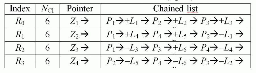
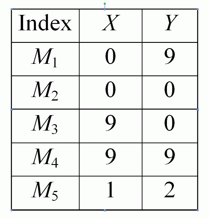
Consider a partition R of an n-dimensional complex A into k-dimensional subcomplexes S_i^k (k=0, 1, ..., n, i=0, 1, ..., m). Subsets with k=0 are some 0-cells of A; each of the subsets with k>0 is combinatorially homeomorphic to an open k-dimensional ball. We define an AC complex B whose cells correspond to the subcomplexes S_i^k . This is the block complex. The cells of B are called block cells, while the subcomplexes S_i^k are the blocks.

Geometric 2D Cell List

The underlying data structure is called a two-dimensional cell list

The image

The sub-list of the 0-block cells contains the coordinates X and Y of each branch point in the original image. This data belong to the "geometric information" enabling the reconstruction of the original image from the cell list. If only topological information is wanted, then the columns with the coordinates can be omitted. The list also indicates for each 0-block cell P_i the number N_lin of all 1-blocks cells incident to P_i and their signed indices. The negative sign of an index L_k in the row of P_i indicates that P_i is the end point of L_k.

The sub-list of lines (1-block cells)	The sub-list of regions (2-block cells)

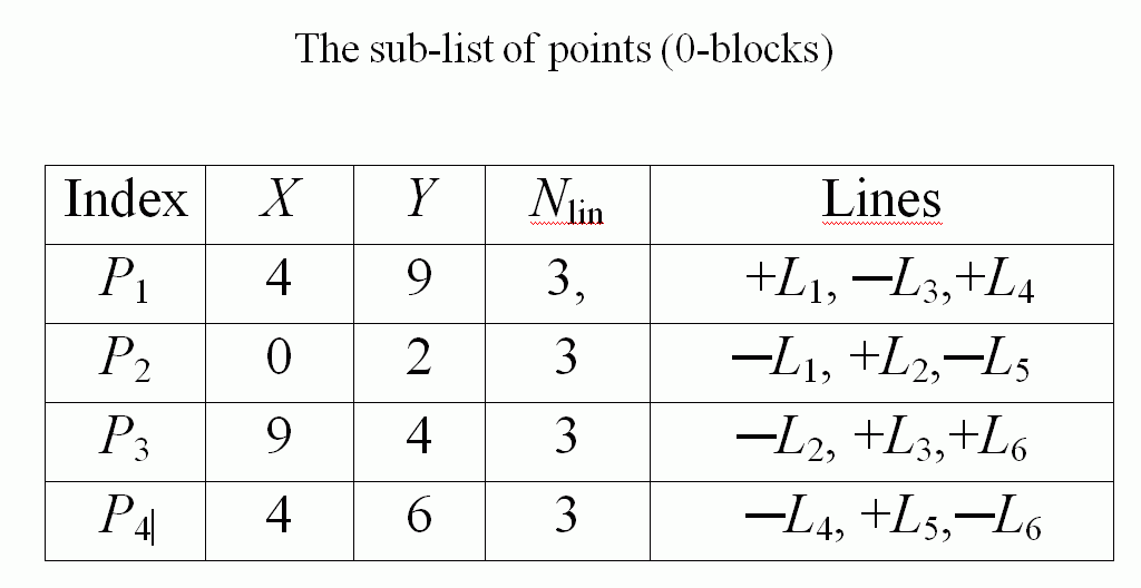
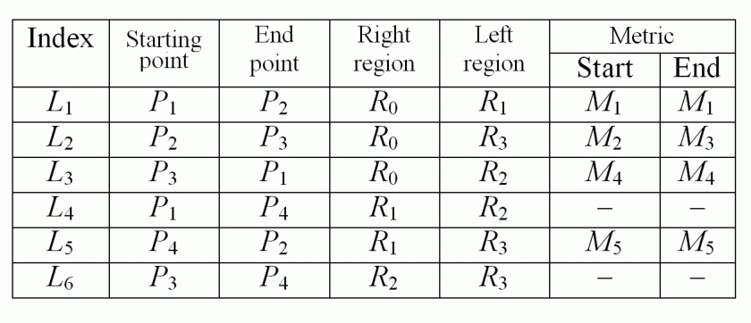
The sub-list of the 1-block cells contains the indices of its startng and end points. It also contains the indices of the right and left regions. The last two columns contain indices of the so-called metric points which are no branch points. Their coordinates are saved in the sub-list of metric data (see below). They are vertices of a polygonal line approximating the corresponding segment of the boundary of a region. The metric points are lying between the end points of a line. They are necessary to describe (together with the coordinates of the branch points) geometric features of the image represented by the block complex and serve for the reconstruction of the image. The coordinates can be omitted in a purely topological version of a cell list.

	The metrical sub-list

It is also possible to make a cell list for a 3D image containing many bodies. If you are interested in details see the refrences [1] and [2]. Here is a simple example

An Example of a 3D Cell List

Small sample with 12 points, 20 lines, 10 faces and 1 body.

Cell List of the small sample with 12 points, 20 lines, 10 faces and 1 body:
----------------- Sub-list of points---------------
Point 1 ( 2; 2; 2) is incident with 3 lines: -1; - 3; - 2;
Point 2 (16; 2; 2) is incident with 3 lines:  1; - 7; - 5;
Point 3 ( 2;16; 2) is incident with 3 lines:  2; - 8; - 4;
Point 4 ( 2; 2; 4) is incident with 4 lines:  3; -13; - 9; -6;
Point 5 (16;16; 2) is incident with 3 lines:  4; -10;   5;
Point 6 (16; 2; 4) is incident with 4 lines:  6; -14; -12;  7;
etc. Points 7 to 12
----------------- Sub-list of lines (Left, Right from outside)
Line  1   StartP= 1   EndP= 1   Left= 2   Right= 1
Line  2   StartP= 1   EndP= 1   Left= 1   Right= 3
Line  3   StartP= 1   EndP= 1   Left= 3   Right= 2
Line  4   StartP= 1   EndP= 3   Left= 1   Right= 5
Line  5   StartP= 1   EndP= 2   Left= 4   Right= 1
Line  6   StartP= 1   EndP= 4   Left= 6   Right= 2
Line  7   StartP= 1   EndP= 2   Left= 2   Right= 4
Line  8   StartP= 1   EndP= 3   Left= 5   Right= 3
Line  9   StartP= 1   EndP= 4   Left= 3   Right= 7
Line 10   StartP= 1   EndP= 5   Left= 4   Right= 5
Line 11   StartP= 1   EndP= 7   Left= 5   Right= 9
Line 12   StartP= 1   EndP= 6   Left= 8   Right= 4
Line 13   StartP= 1   EndP= 4   Left= 7   Right= 6
Line 14   StartP= 1   EndP= 6   Left= 6   Right= 8
Line 15   StartP= 1   EndP= 9   Left=10   Right= 6
Line 16   StartP= 1   EndP= 7   Left= 9   Right= 7
Line 17   StartP= 1   EndP= 9   Left= 7   Right=10
Line 18   StartP= 1   EndP= 8   Left= 8   Right= 9
Line 19   StartP= 1   EndP=11   Left= 9   Right=10
Line 20   StartP= 1   EndP=10   Left=10   Right= 8
----------------- Sub-list of 10 faces ---------------
Face  1   Boundary: (P 2; L - 1) (P 1: L   2) (P 3: L   4) (P 5: L - 5)
Face  2   Boundary: (P 4; L - 3) (P 1: L   1) (P 2: L   7) (P 6: L - 6)
Face  3   Boundary: (P 3; L - 2) (P 1: L   3) (P 4: L   9) (P 7: L - 8)
Face  4   Boundary: (P 2; L   5) (P 5: L  10) (P 8: L -12) (P 6: L - 7)
Face  5   Boundary: (P 5; L - 4) (P 3: L   8) (P 7: L  11) (P 8: L -10)
Face  6   Boundary: (P 4; L   6) (P 6: L  14) (P10: L -15) (P 9: L -13)
Face  7   Boundary: (P 7; L - 9) (P 4: L  13) (P 9: L  17) (P11: L -16)
Face  8   Boundary: (P 6; L  12) (P 8: L  18) (P12: L -20) (P10: L -14)
Face  9   Boundary: (P 8; L -11) (P 7: L  16) (P11: L  19) (P12: L -18)
Face 10   Boundary: (P11; L -17) (P 9: L  15) (P10: L  20) (P12: L -19)
----------------- Sub-list of 1 body ---------------
Faces 1, 2, 3, 4, 5, 6, 7, 8, 9, 10.

The image can be exaclty reconstructed from its cell list. The idea of the reconstruction is represented in the lecture 'Simple Algorithms Based on Digital Topology'.

If you are interested in details see the reference [1] and take the book: 'Geometry of Locally Finite Spaces'.

References

[1] V.Kovalevsky, Finite Topology as Applied to Image Analysis, Computer Vision, Graphics and Image Processing, v. 46, pp. 141-161, 1989..

[2] V. Kovalevsky: Geometry of Locally Finite Spaces, Monography, Berlin 2008.

Download: Print version

top of page:

Last update: October 24, 2011