Curvature of curves
www.kovalevsky.de, last update: October 26, 2011
 Let me know
what you think
| Home | Index of Lectures | << Prev | Next >> | PDF Version of this Page |
Curvature of curveswww.kovalevsky.de, last update: October 26, 2011 |
|
Let me know what you think |
|
|
The curvature radius R: The limit of the radius of a circle running through three points of the curve, when the distance between
the points tends to zero. The curvature C = 1/R.
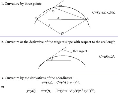 |
The curvature of a curve in a 2D space is defined in analytical geometry by means of derivatives of the function describing the
curve. In digital images curves are defined in a grid. The function describing a curve takes discrete values, e.g. integer values.
How can one compute derivatives of such functions ?
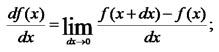 | Consider the definition of the first derivative of a function of a single variable: |
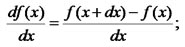 | What will happen, if we try to compute the value by the computer while taking dx equal to the smallest number representable in the computer ? |
| An attempt to estimate the derivative of y=x2 as dy/dx with the smallest possible value of Δx. | |||
| Looks well |  | Small distortions | |
| Large distortions |  | Crasy values |
The estimate of the first derivative
E1 = (f(x+Δx)−f(x−Δx)/
(2*Δx);
The values of f(x) cannot be computed exactly; they contain a computation error of ε. We consider the values of
f(x+Δx)+ε, f(x−Δx)+ε and represent
f(x+Δx) and f(x−Δx by the Taylor formula.
E1= [f(x)+f '(x)*Δx +
0.5*f "(x)·Δx2+(1/6)·f (3)
(x+k*Δx)*Δx3−
f(x)−f '(x)*Δx +
0.5*f "(x)·Δx2−(1/6)·f (3)
(x+k*Δx)*Δx3−
where k,m∈[0, 1], F3 is the average value of the third derivative of f(x) in the interval
(x−Δx, x+Δx) and ε is the estimate of the possible error of computing
the values of f(x).
The error Er of the estimation E1:
Er = (1/6)*F3*Δx2 + ε/Δx;
(1)
We find the optimal value of Δx while setting the partial derivative of (1) with respect to Δx equal
to 0 and receive:
optim Δx = (3*ε/F3)1/3;
minimum Error = ((1/6)*32/3+3-1/3)*
ε2/3*F31/3 ~=
1.04*ε2/3*F31/3.
We obtain in a similar way the error in estimating the second derivative of f(x), the optimal value of
Δx:
optim Δx = (48*ε/F4)1/4
and the minimum error:
minimum Error = ((1/12)*481/2+4*48−1/2)*ε1/2*
F41/2 ~= 1.15*(ε*F4)1/2.
(2)
Estimates F3 and F4< of the third and fourth derivatives are respectively:
F3 ≈ (f(x+2*Δx)−2·f(x+Δx)+2*f(x−Δx)−
f(x−2*Δx) )/(2*Δx3);
F4 ≈ (f(x+2*Δx)−4·f(x+Δx)+6*f(x)−
4*f(x−Δx)+f(x−2*Δx) )/Δx4.
(3)
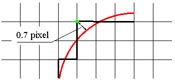
| A modest demand: the curvature error ≤10%; coordinate error |
 |
| top of page: |